hist(cdc$height, col = 'lightskyblue', main = '', xlab = 'Height')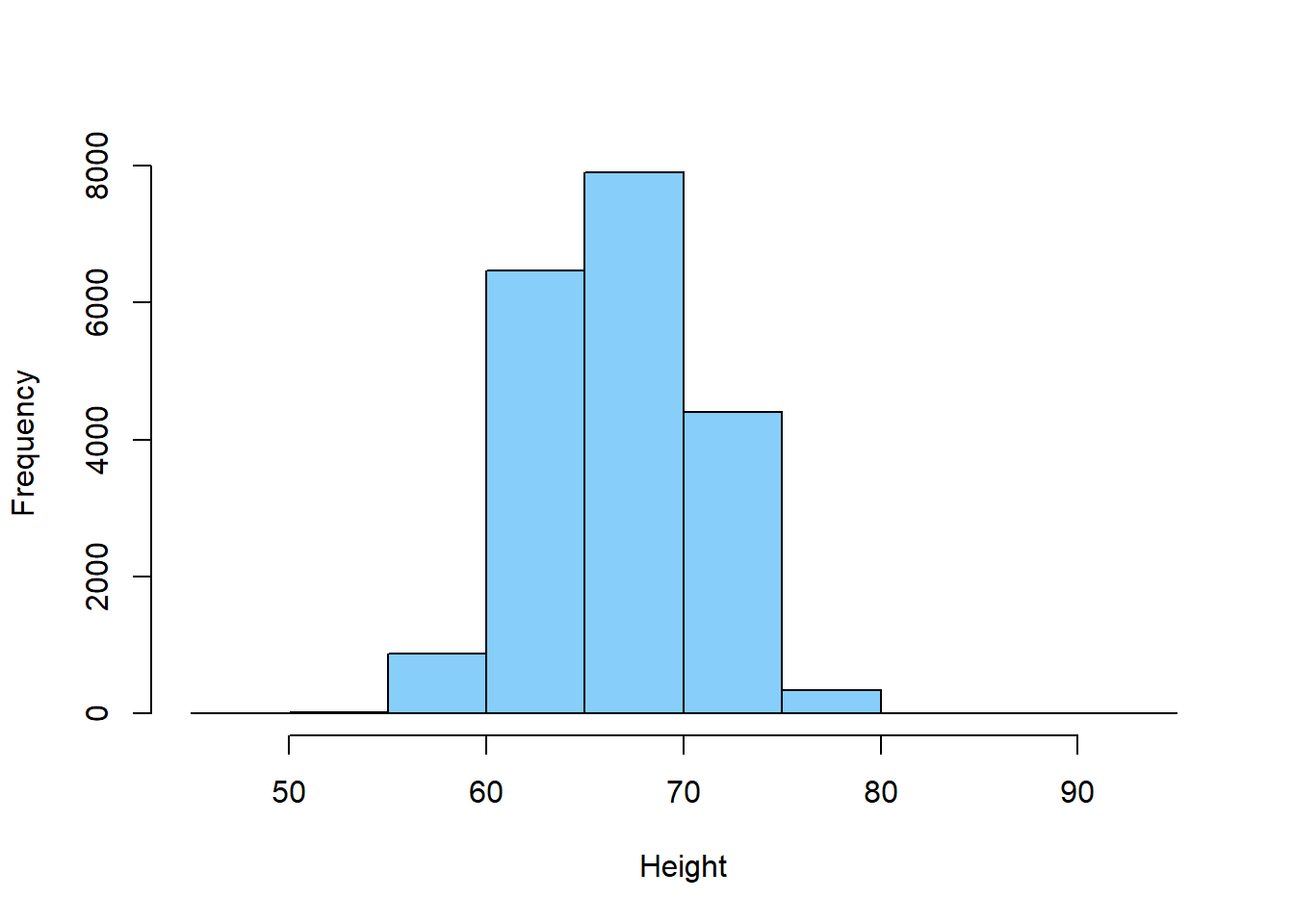
hist(cdc$weight, col = 'salmon', main = '', xlab = 'Weight')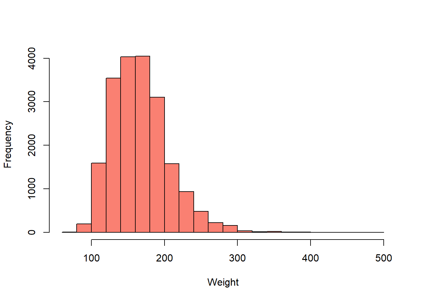
hist(cdc$age, col = 'olivedrab3', main = '', xlab = 'Age')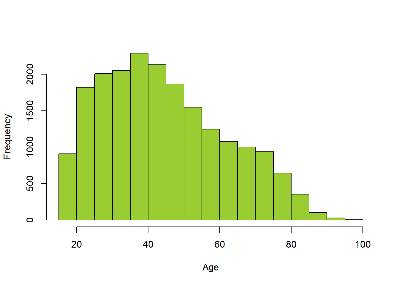
The data set is slightly modified from OpenIntro,
The Behavioral Risk Factor Surveillance System (BRFSS) is an annual telephone survey of 350,000 people in the United States collected by the Centers for Disease Control and Prevention (CDC). As its name implies, the BRFSS is designed to identify risk factors in the adult population and report emerging health trends. For example, respondents are asked about their diet and weekly physical activity, their HIV/AIDS status, possible tobacco use, and even their level of healthcare coverage. The BRFSS Web site contains a complete description of the survey, the questions that were asked and even research results that have been derived from the data.
This data set is a random sample of 20,000 people from the BRFSS survey conducted in 2000. While there are over 200 questions or variables in this dataset, this data set only includes 9 variables.
The data set has the following variables:
genhlth - General health, with categories Excellent, Very Good, Good, Fair, and Poor
exerany - Whether the respondent exercised in the past month
hlthplan - Whether respondent has some form of health coverage
smoke100 - Whether respondent has smoked at least 100 cigarettes in their entire life
height - Respondent’s height in inches
weight - Respondent’s weight in pounds
wtdesire - Respondent’s desired weight in pounds
age - Respondent’s age in years
gender - Respondent’s gender
The hands-on activities below are adapted from the Introduction to data lab developed by Dr. Andrew Bray.
💻 Hands-On
Describe the data distributions of variables height, weight, and age in the cdc data set.
Looking at their histograms, the data distribution of height is symmetric, whereas the data distributions of weight and age are right-skewed.
hist(cdc$height, col = 'lightskyblue', main = '', xlab = 'Height')
hist(cdc$weight, col = 'salmon', main = '', xlab = 'Weight')
hist(cdc$age, col = 'olivedrab3', main = '', xlab = 'Age')
💻 Hands-On
Obtain numerical summaries and box plots of height, weight, and age in the cdc data set.
Note that there are very extreme values of weight. Some people are very malnourished while some are heavier than the common belief. This can be the nature of the data or there are errors. It is best to consult someone with domain expertise if further analyses are needed.
summary(cdc$height) Min. 1st Qu. Median Mean 3rd Qu. Max.
48.00 64.00 67.00 67.18 70.00 93.00 boxplot(cdc$height, col = 'lightskyblue', horizontal = TRUE, xlab = 'Height')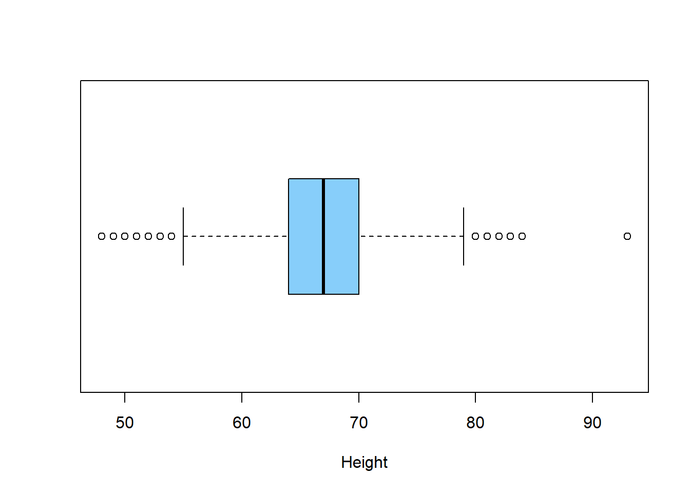
summary(cdc$weight) Min. 1st Qu. Median Mean 3rd Qu. Max.
68.0 140.0 165.0 169.7 190.0 500.0 boxplot(cdc$weight, col = 'salmon', horizontal = TRUE, xlab = 'Weight')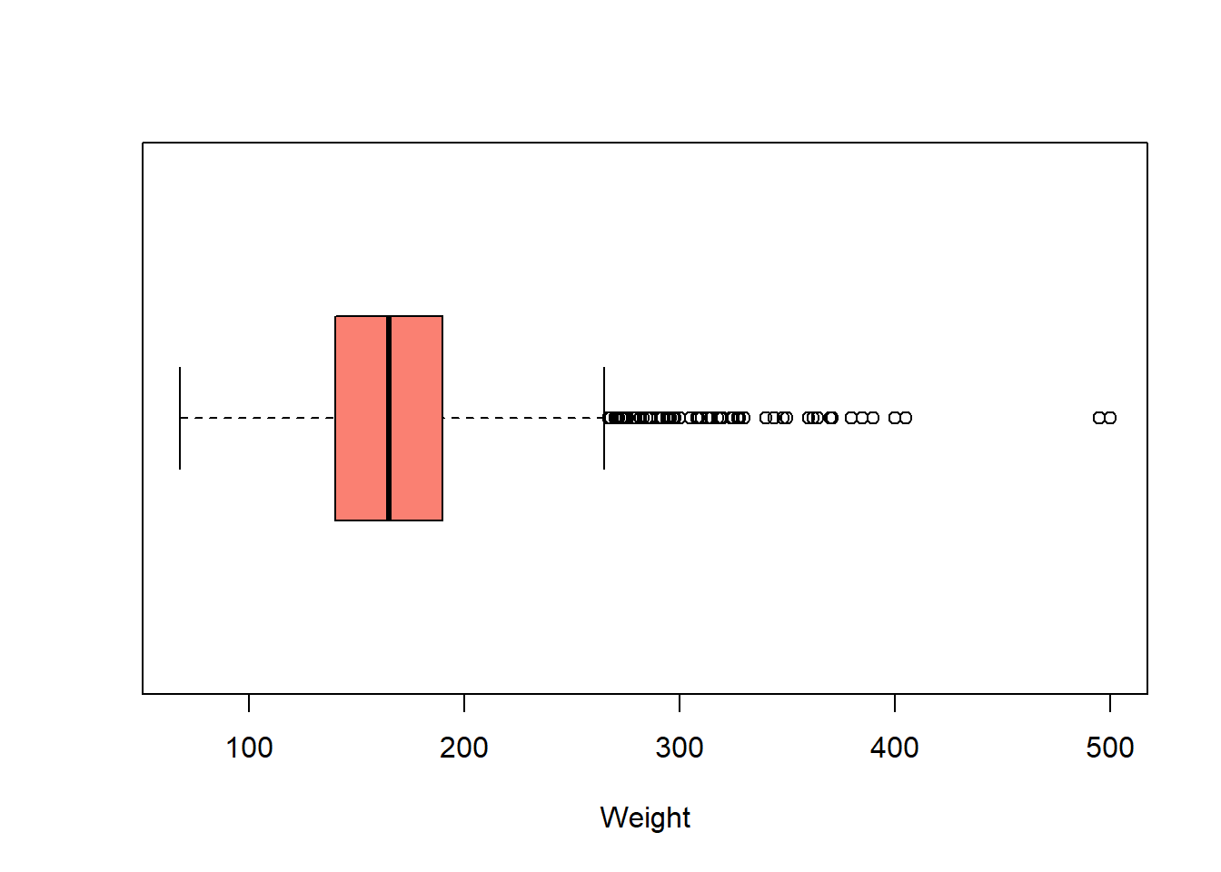
summary(cdc$age) Min. 1st Qu. Median Mean 3rd Qu. Max.
18.00 31.00 43.00 45.07 57.00 99.00 boxplot(cdc$age, col = 'olivedrab3', horizontal = TRUE, xlab = 'Age')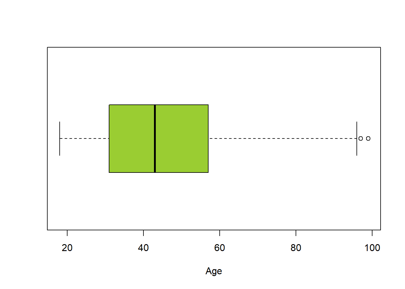
💻 Hands-On
Compare height and weight of male and female individuals.
boxplot(height ~ gender, data = cdc, pch = 16, col = c('royalblue1', 'indianred1'))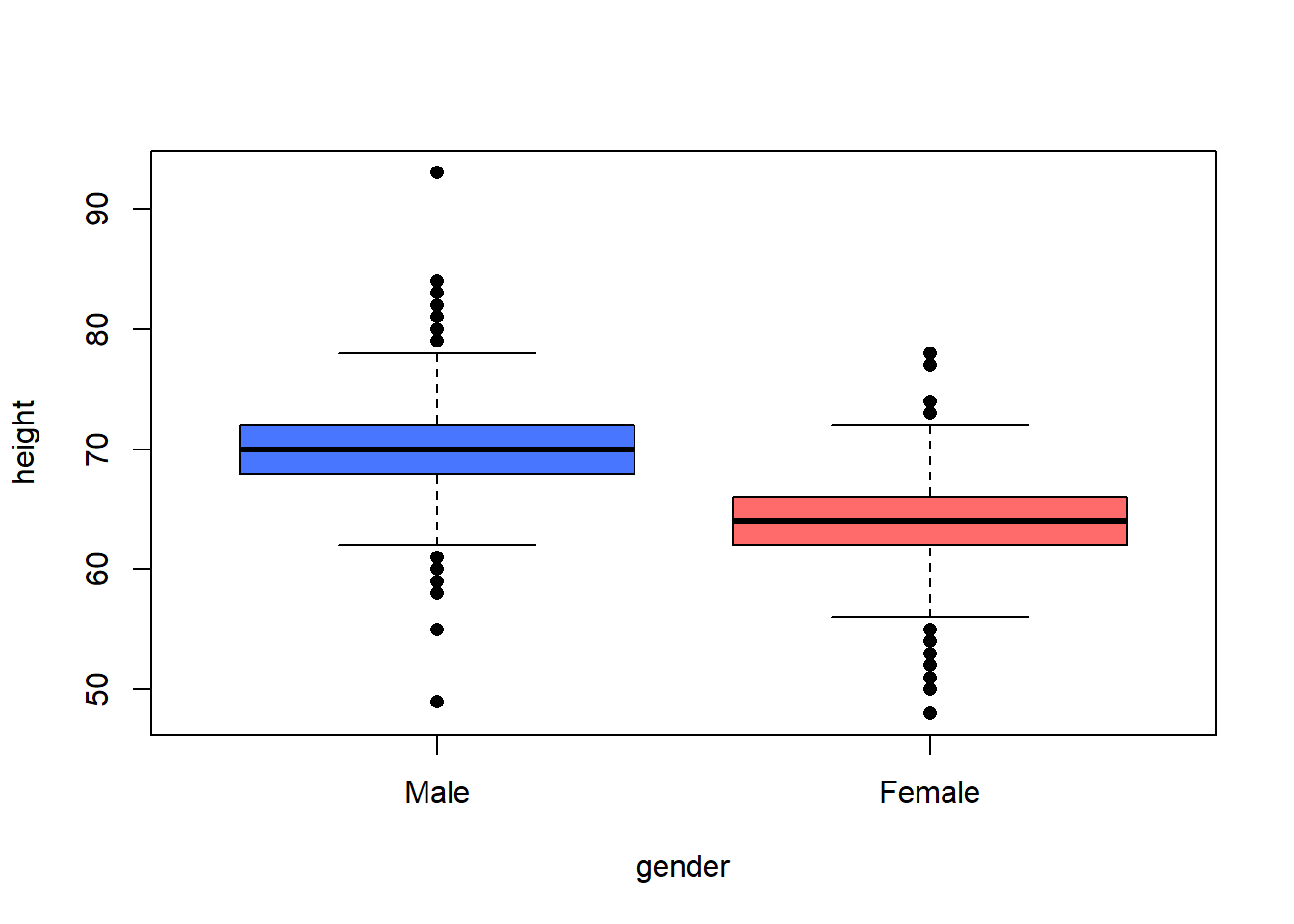
boxplot(weight ~ gender, data = cdc, pch = 16, col = c('royalblue1', 'indianred1'))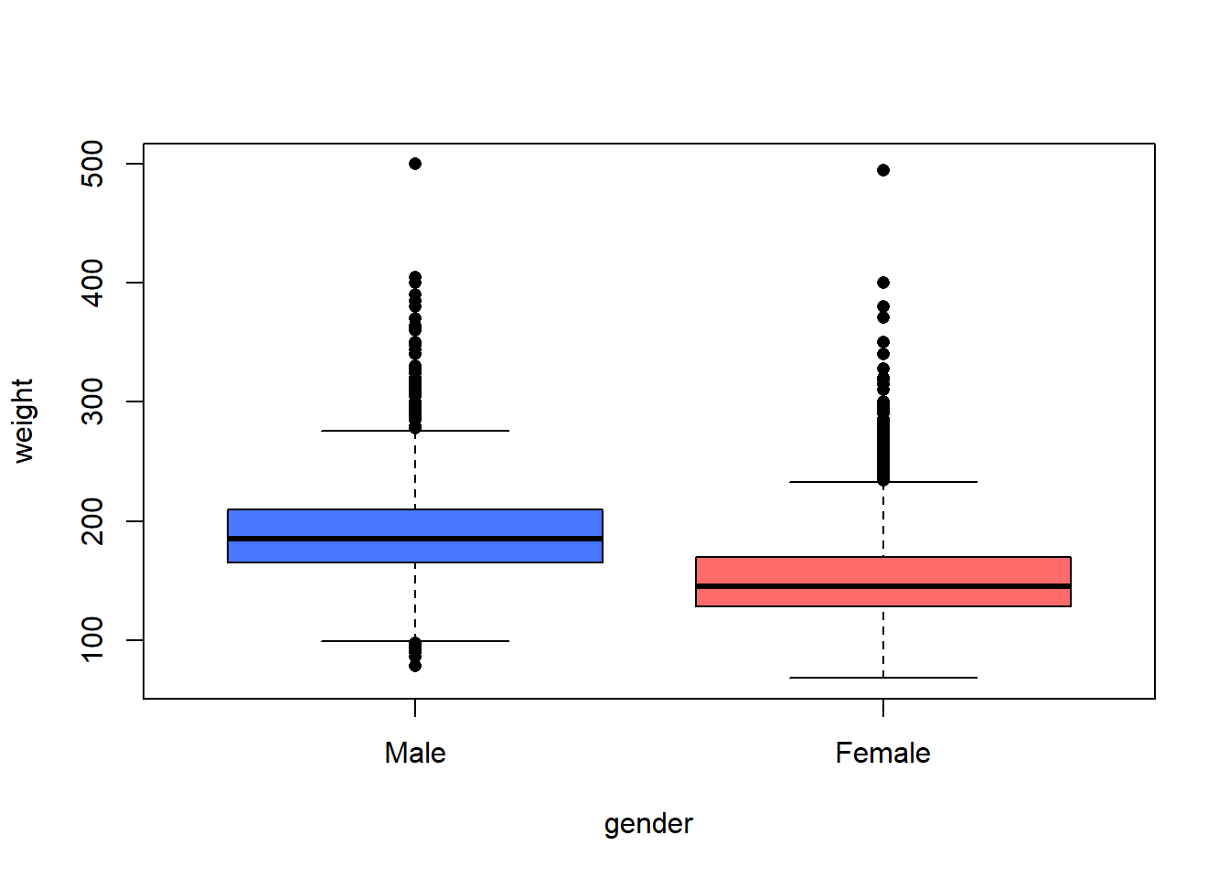
💻 Hands-On
Add a new variable bmi to the cdc data set to represent body mass index (BMI).
\[ \text{BMI} = \dfrac{\text{weight}~(\text{lb})}{\text{height}~(\text{in})^2} \times 703 \]
cdc$bmi <- (cdc$weight / cdc$height^2) * 703💻 Hands-On
According to standard guidelines, BMI is categorized as underweight (less than 18.5), healthy (between 18.5 and 24.9), overweight (between 25 and 29.9), and obese (30 or higher). How many people are considered underweight in the data set? How many people are considered healthy in the data set?
The number of people who are considered underweight is
sum(cdc$weight < 18.5)[1] 0The number of people who are considered healthy is
sum(cdc$weight >= 18.5 & cdc$weight <= 24.9)[1] 0💻 Hands-On
Obtain the correlation and scatter plot of weight and desired weight wtdesire.
The correlation of weight and desired weight wtdesire is strongly positive, meaning these measures tend to go in the same direction. However, it is not very clear whether people tend to like gaining or losing weights.
cor(cdc$weight, cdc$wtdesire)[1] 0.8000521The scatter plot of weight and desired weight wtdesire is given below.
plot(cdc$weight, cdc$wtdesire, pch = 16, cex = 0.8, col = 'goldenrod1',
     xlab = 'Current Weight', ylab = 'Weight Desired',)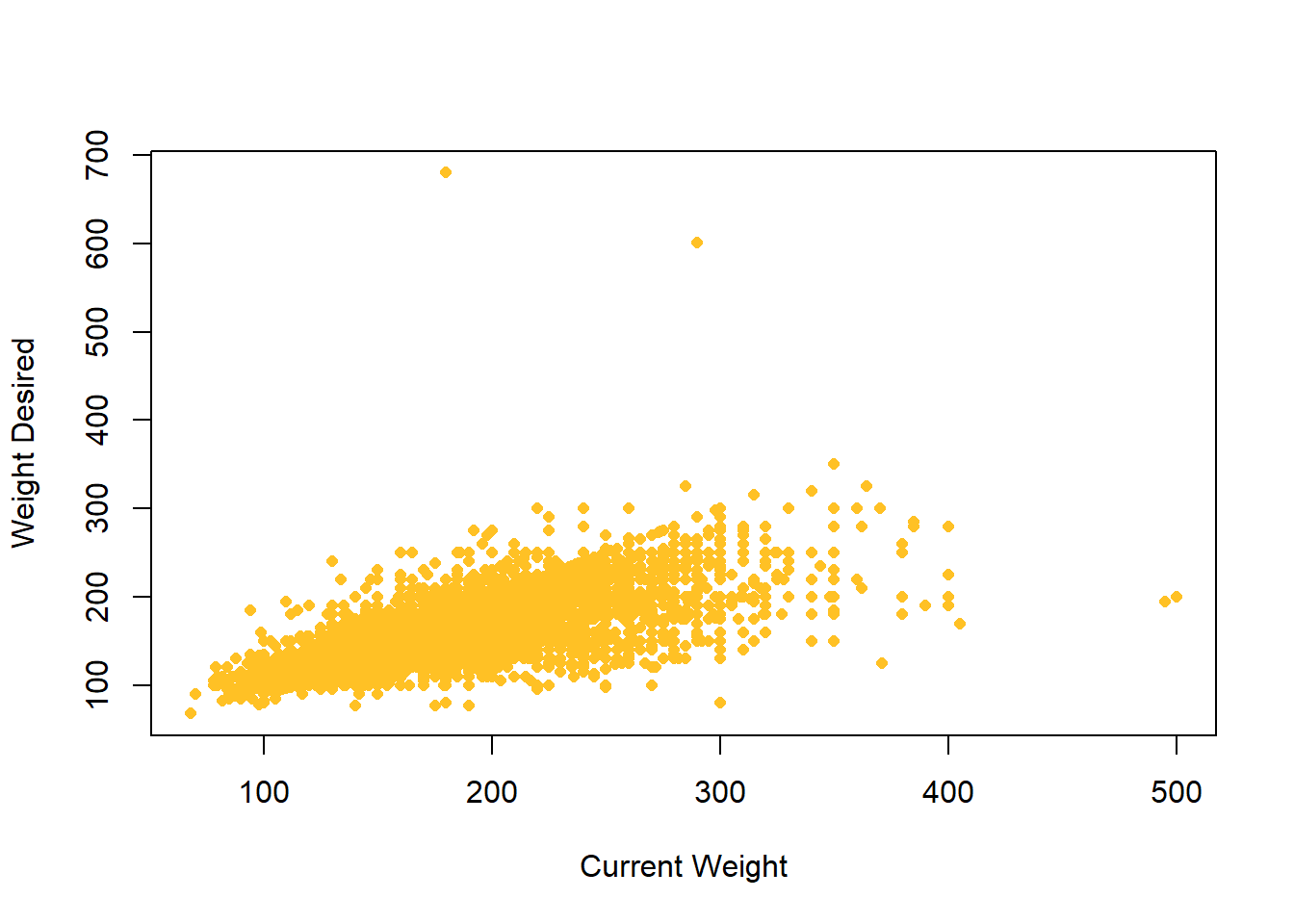
💻 Hands-On
Add a new variable wdiff to the cdc data set to represent the difference between desired weight wtdesire and current weight weight.
Note that a positive wdiff implies that the person wants to gain weight and a negative wdiff implies that the person wants to lose weight.
cdc$wdiff <- cdc$wtdesire - cdc$weight💻 Hands-On
Describe the data distribution of wdiff in the cdc data set.
Most wdiff concentrate below 0, meaning people tend to want to lose weight than to gain weight.
hist(cdc$wdiff, col = 'hotpink2', main = '', xlab = 'Weight Difference')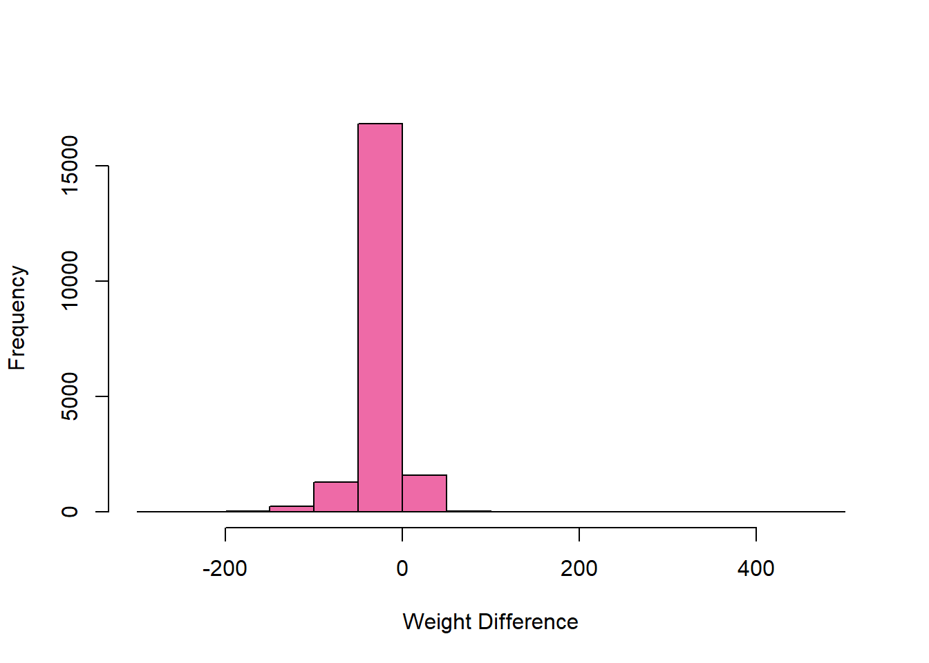
💻 Hands-On
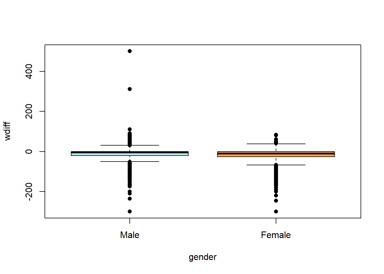
Compare wdiff of male and female individuals. What conclusion can you make about how people feel about their current weight?
The side-by-side box plots indicate comparable wdiff between male and female individuals. Most values are below zero. From this data set, it seems like people regardless of their gender tend to want to lose weight.
boxplot(wdiff ~ gender, data = cdc, pch = 16, col = c('paleturquoise', 'tan1'))