Dimensionality reduction refers to the process of reducing the number of variables or transforming the original variables into a smaller set of new variables.
Dimensionality reduction is unsupervised because different methods reduce dimensionality based on different criteria:
Principal component analysis seeks to capture as much variability in the data set as possible.
Linear discriminant analysis reduces dimensionality so that the separation between groups is maximized.
Multidimensional scaling preserves relative distances between observations when reducing dimensionality.
From mlguru.ai
Principal component analysis
Principal component analysis (PCA) aims to explain the variability of a multivariate dataset using a few special linear combinations of the original variables \(X_1, X_2, \dots, X_p\) called principal components.
Principal component analysis is arguably the most popular dimensionality reduction method.
A data set with \(p\) variables is transformed into a data set with \(p\) principal components. Each principal component refers to a new direction or axis that captures as much variability as possible.
Although \(p\) components are required to reproduce the total variability, using the first few principal components is enough to explain most of this variability.
Geometrically, a linear combination of \(p\) variables \(X_1, X_2, \dots, X_p\) defines a new direction or axis. \[a_1 X_1 + a_2 X_2 + \dots + a_p X_p \]
A linear combination of \(p = 2\) variables \(X_1\) and \(X_2\) may define a new axis as follows
A linear combination of \(p = 3\) variables \(X_1, X_2\), and \(X_3\) may define a new axis as follows
For a two-dimensional data set, we look for a linear combination \(a_1 X_1 + a_2 X_2\) that captures the most variability.
Many linear combinations (new axes) are available, but the amount of variability they capture varies.
The linear combination (axis) that captures the most variability is the first principal component.
Another linear combination (axis) that captures most of the remaining variability is the second principal component.
The first principal component is the linear combination of \(X_1, X_2, \dots, X_p\) that captures the most variability the data set.
The second principal component is the linear combination \(X_1, X_2, \dots, X_p\) that is uncorrelated with the first principal component and captures most of the remaining variability.
The \(j\)th principal component is the linear combination \(X_1, X_2, \dots, X_p\) that is uncorrelated with all previous principal components and captures most of the remaining variability.
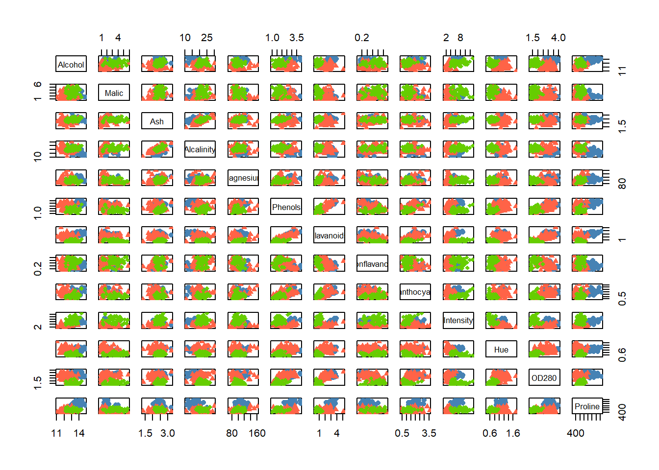
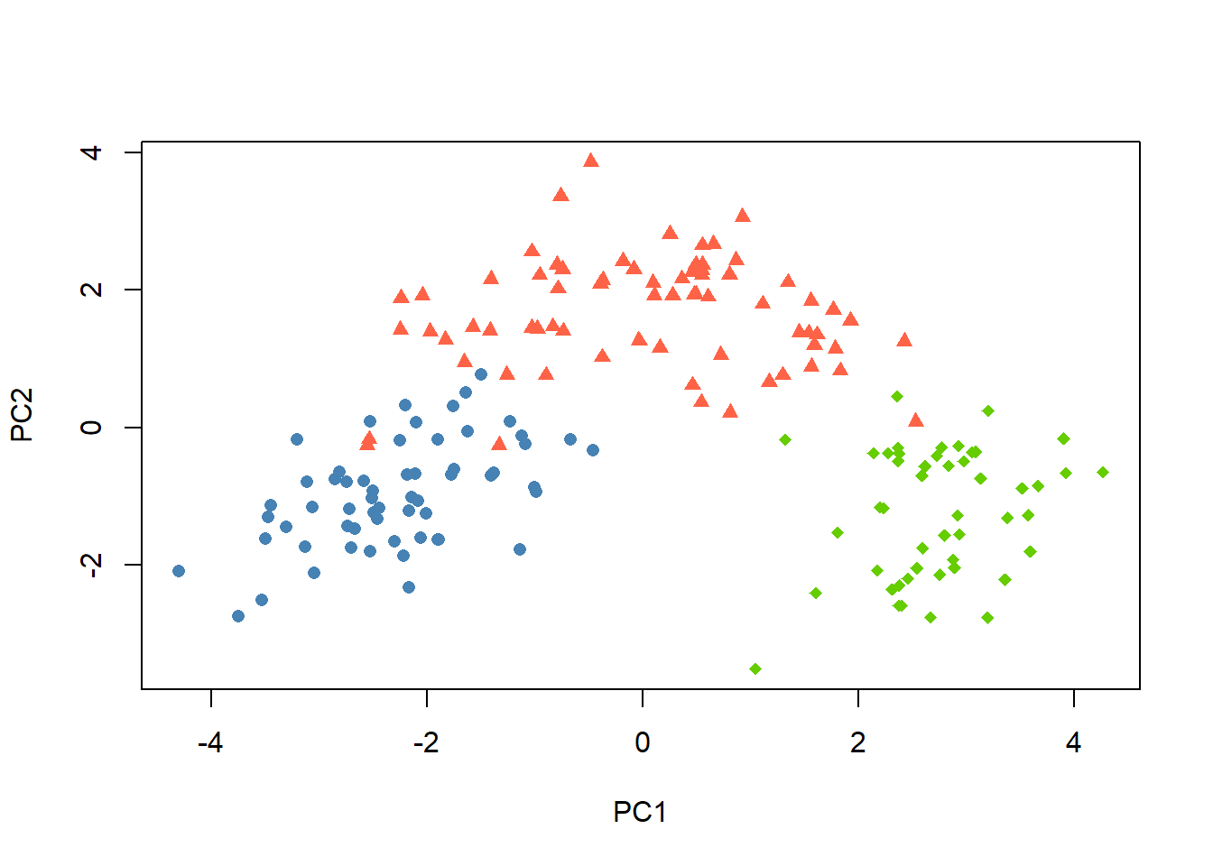
The Italian wine data set contains a sample of \(178\) bottles: Barolo, Grignolino, and Barbera. For each bottle, the following \(13\) chemical and physical properties are measured: Alcohol, Malic, Ash, Alcalinity, Magnesium, Phenols, Flavanoids, Nonflavanoid, Proanthocyanins, Intensity, Hue, OD280, Proline.
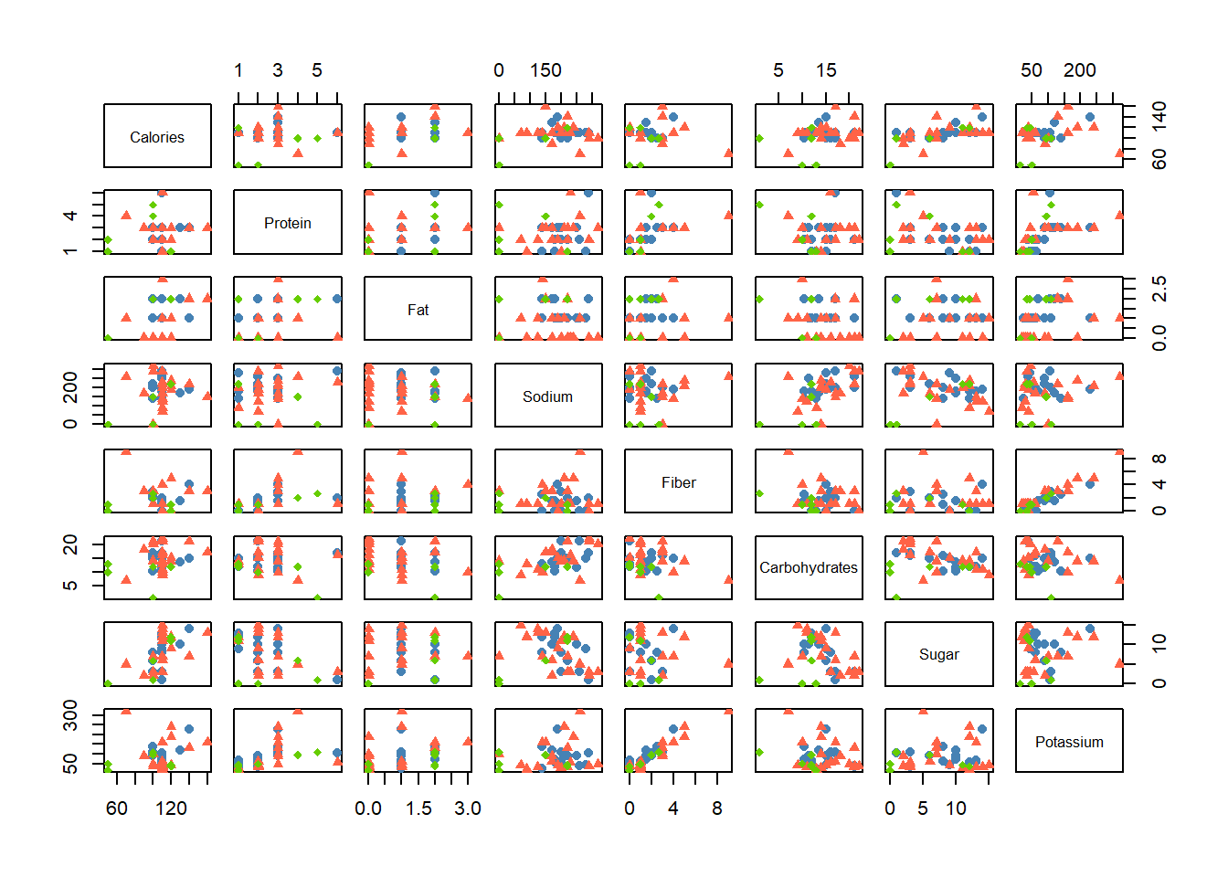
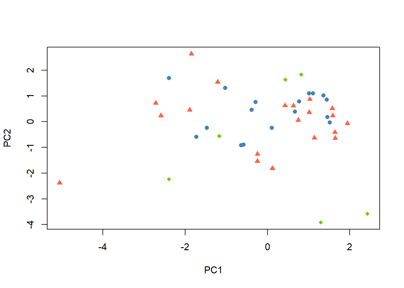
In the cereal data set, there are breakfast cereals produced by three different American manufacturers: General Mills (G), Kellogg (K), and Quaker (Q). Conduct a principal component analysis on the data set. Produce the first two principal component scores and visualize them on a two-dimensional scatter plot. Use different colors and plotting symbols to identify the three manufacturers.
Answer
load(url('https://github.com/hungtong/DS-01-101/raw/refs/heads/main/dataset/cereal.rdata'))X <- cereal[, -(1:2)]pairs(X, col = cols[cereal$Manufacturer], pch = pchs[cereal$Manufacturer])