10: k-Means Clustering

Readings

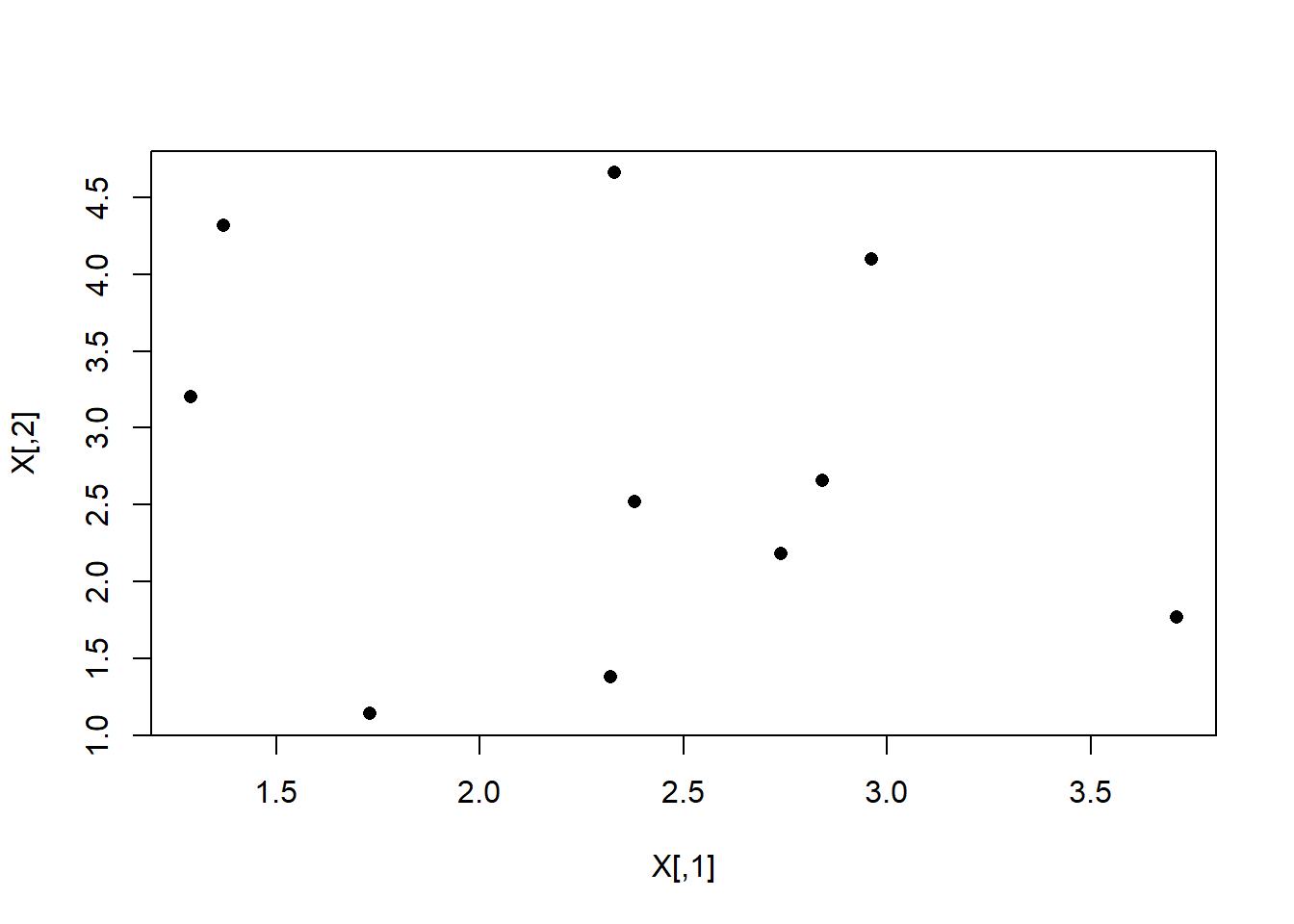
From An Introduction to Statistical Learning with Applications in R by Drs. Gareth James, Daniela Witten, Trevor Hastie, and Rob Tibshirani:

Unsupervised Learning

The book is freely available at https://www.statlearning.com/

Also, check out the following videos:

Topics

k-Means Clustering
Clustering Methods

Clustering

Recall that classification aims to assign an observation to known category or class. On the other hand, clustering aims to find smaller groups of similar observations.
The notion of similarity is largely defined by the practitioners rather than known labels. Thus, clustering is said to be unsupervised.

Examples of clustering include:
- Customer segmentation to identify purchasing patterns.
- Grouping genes with similar expression levels.
- Color quantification and text mining.

k-Means clustering

The most popular clustering method for numerical data is arguably \(k\)-means clustering. In \(k\)-means clustering, members of a cluster should be well represented by its cluster mean, because the cluster mean minimizes the sum of squared distances to all observations in its cluster.

Recall that the Euclidean distance is a popular distance measure between two numerical observations \((x_1, x_2, \dots, x_p)\) and \((y_1, y_2, \dots, y_p)\)

\[\sqrt{ (x_1 - y_1)^2 + (x_2 - y_2)^2 + \dots + (x_p - y_p)^2 }\]
\(k\)-means clustering is done as follows:
- Randomly select \(k\) observations as the initial cluster centroids (means).
- Go through all observations and assign an observation to the cluster whose centroid (mean) is nearest.
- With all cluster memberships determined, recalculate the cluster centroids (means).
- Repeat the previous two steps until no reassignments take place.
Consider the following data set that we want to find groups of similar observations with \(k\)-means clustering.

Suppose we want to find \(k = 3\) groups. We will randomly select \(3\) observations to be the cluster means. Each cluster mean represents a group. We have red triangle, green diamond, and blue square.

We then go through every observation in the data set. Specifically, we compute the distance between this observation to each of the \(3\) cluster means. The observation will have the membership of the nearest cluster mean. Below, the observation is assigned to the green diamond group because the green diamond cluster mean is nearest to it.

We then go to the next observation and repeat the above process. This observation is assigned to the red group because the red triangle cluster mean is nearest to it.

Another observation is assigned to the green diamond group because the green diamond cluster mean is nearest to it.

Another observation to the green diamond cluster.

The next observation is assigned to the blue square group because the blue square cluster mean is nearest to it.

We repeat the above process for all observation.s

Once we have all the cluster memberships, we will compute the new cluster means. Recall that we randomly selected observations to be the cluster means. Thus, the new cluster means hopefully represent the groups better.

With the new cluster means, we will go through all observations in the data set again to assign cluster memberships based on the nearest cluster means.

After going through all observations, we will have new cluster memberships,

Then, we update the cluster means. The algorithm will stop until the change in cluster means is minimal.

The final cluster memberships will be dependent upon the initial partition. Thus, it is recommended to rerun the algorithm multiple times and select the best solution.

X <- matrix(nrow = 10, ncol = 2, byrow = TRUE, c(
  2.33, 4.66, 
  2.96, 4.10,
  3.71, 1.77,
  1.29, 3.20,
  1.73, 1.14,
  1.37, 4.32,
  2.32, 1.38,
  2.38, 2.52,
  2.74, 2.18,
  2.84, 2.66
))

plot(X, pch = 16)

The function kmeans() can be used for clustering. Note that since \(k\)-means clustering involves random initialization, to make the solution more stable, we can specify a higher number of random sets to start.

km <- kmeans(X, centers = 3, nstart = 5)

plot(X, pch = 16, col = km$cluster)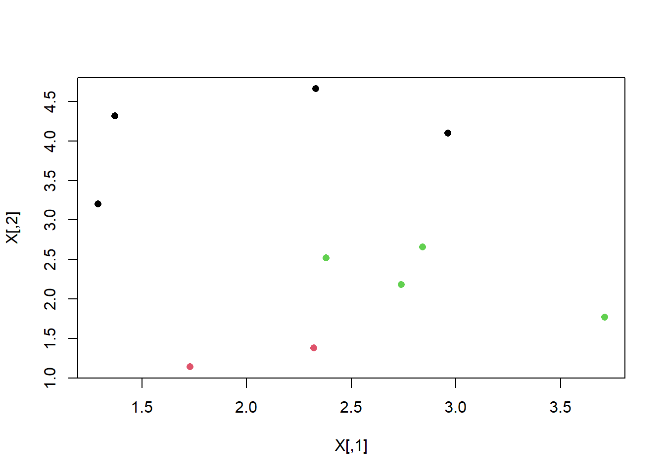

Consider the faithful data set that records waiting time between eruptions and the duration of the eruption for the Old Faithful geyser in Yellowstone National Park, Wyoming, USA.

plot(faithful, pch = 16)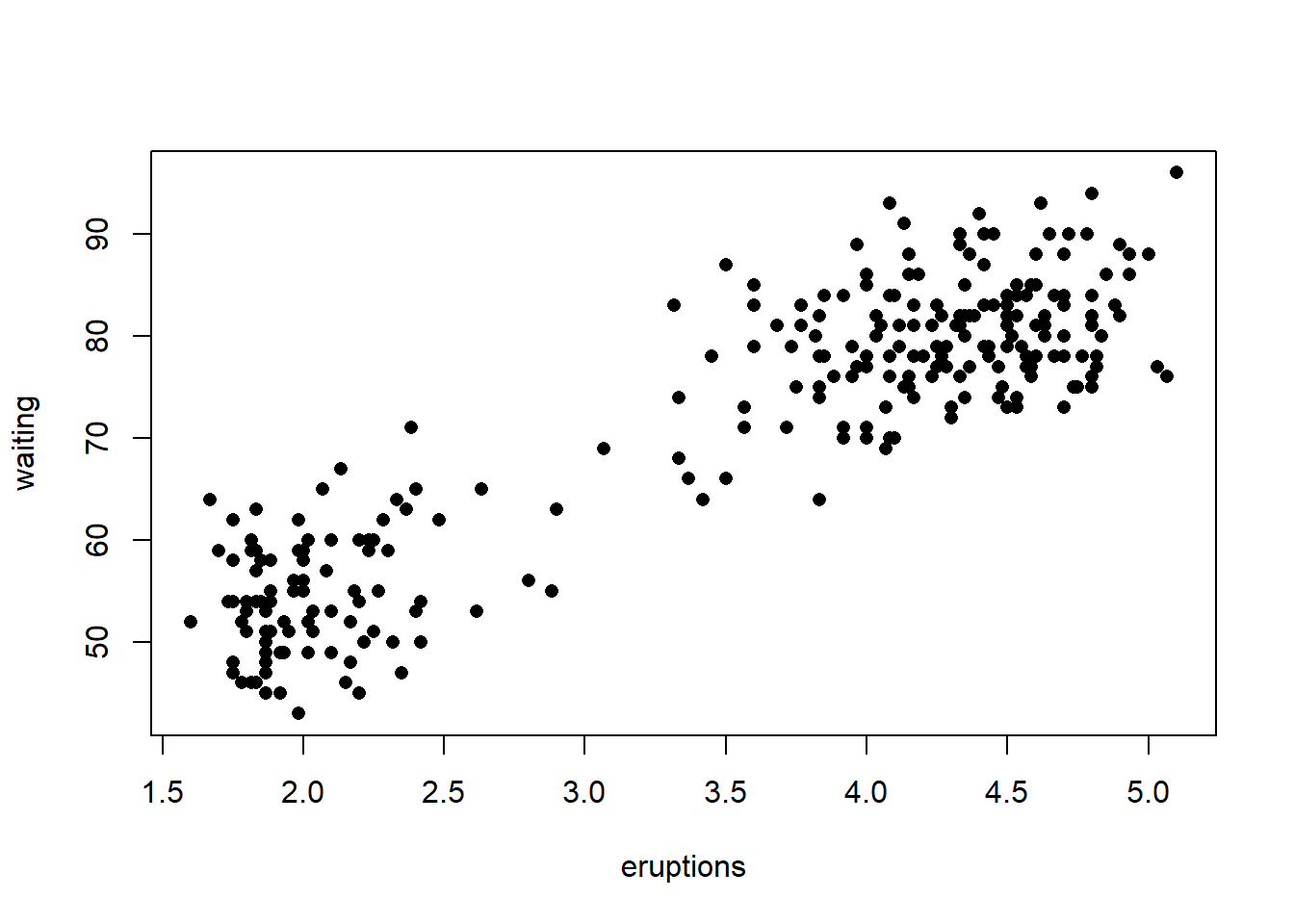

library(cluster)

km2 <- kmeans(faithful, centers = 2, nstart = 5)
plot(faithful, pch = 16, col = km2$cluster)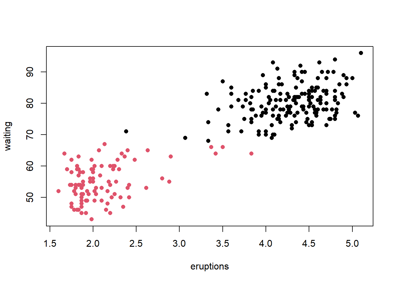

km3 <- kmeans(faithful, centers = 3, nstart = 5)
plot(faithful, pch = 16, col = km3$cluster)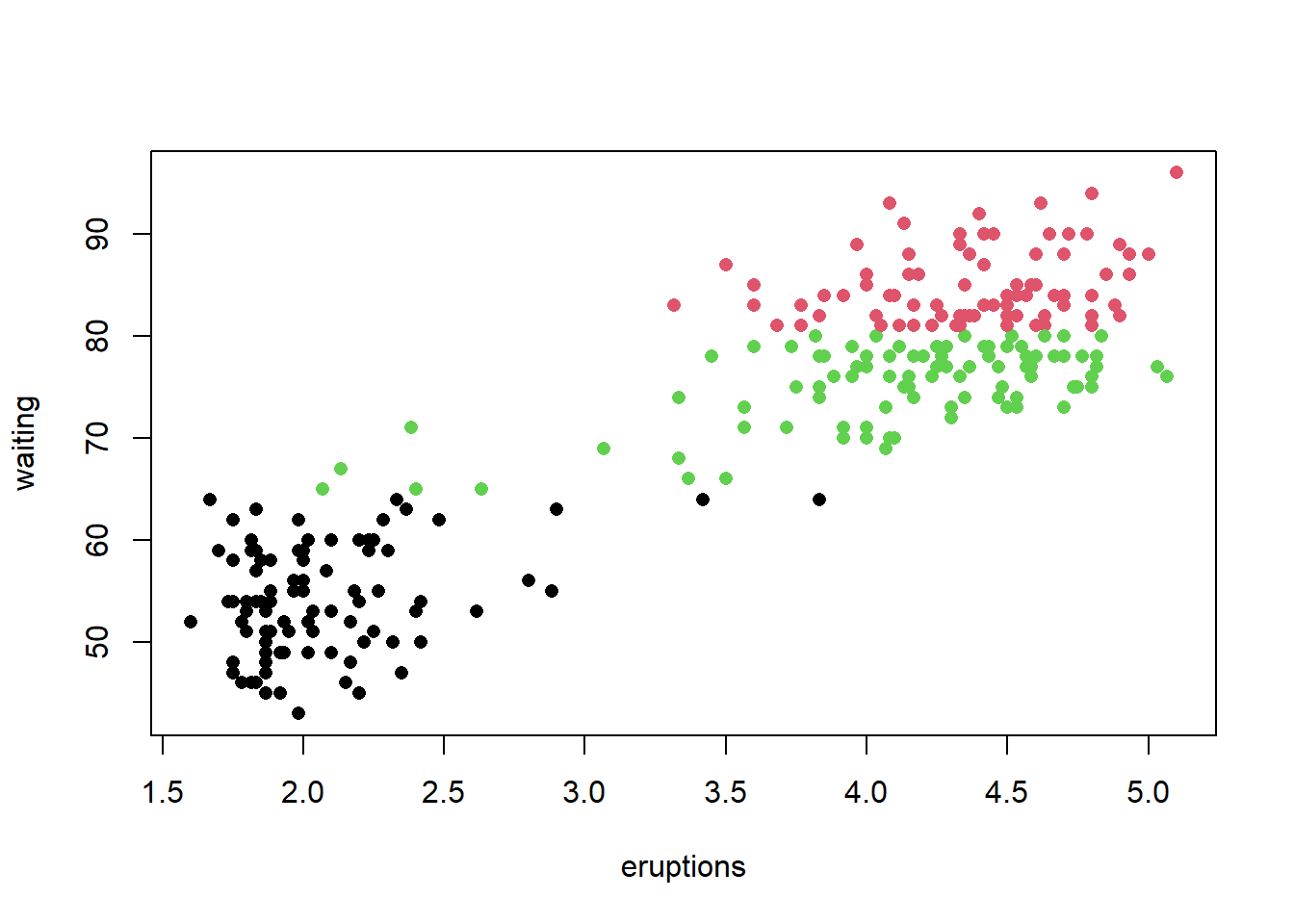

km4 <- kmeans(faithful, centers = 4, nstart = 5)
plot(faithful, pch = 16, col = km4$cluster)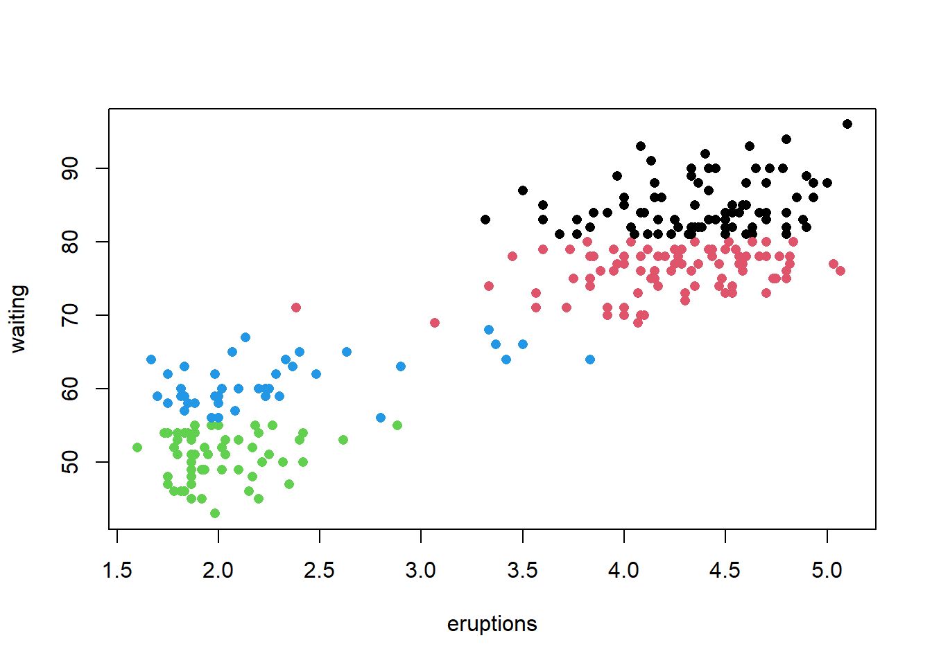

km5 <- kmeans(faithful, centers = 5, nstart = 5)
plot(faithful, pch = 16, col = km5$cluster)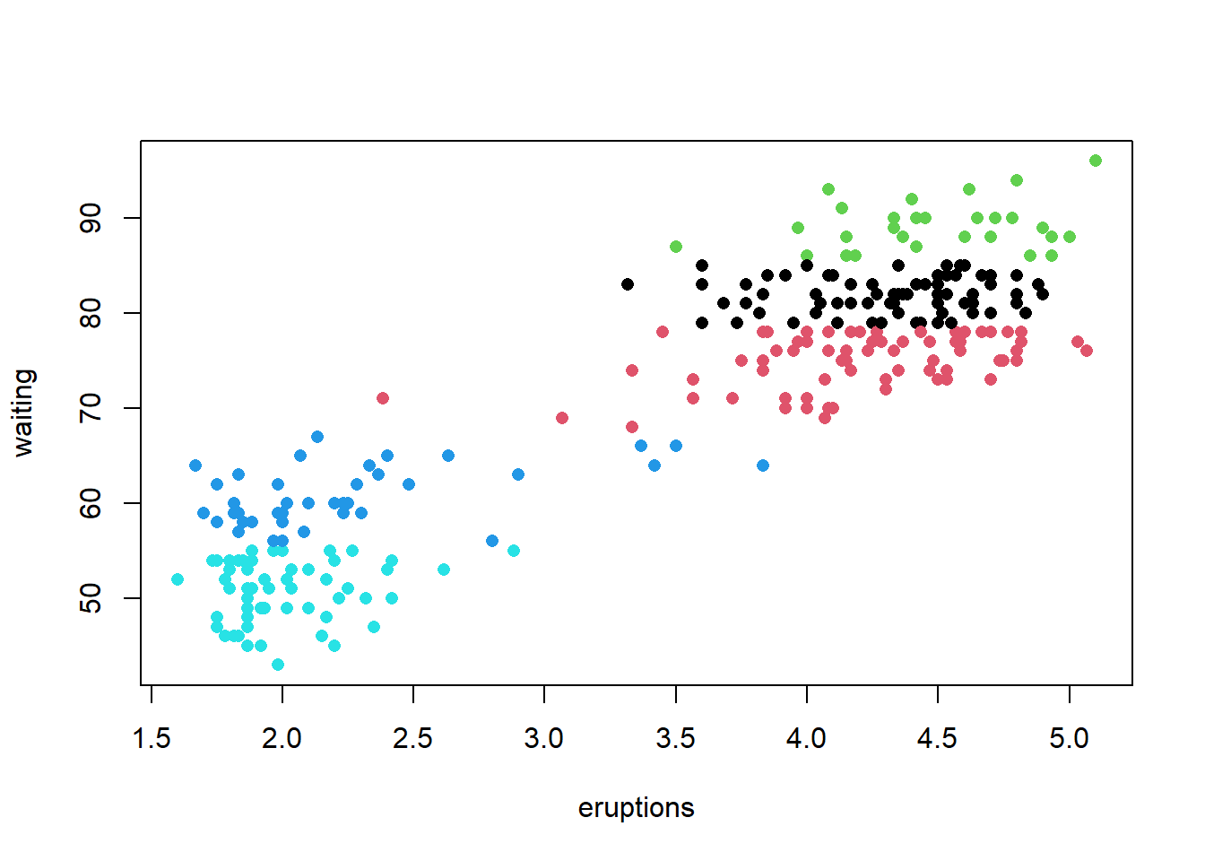

Choosing the number of clusters \(k\) is an important decision in cluster analysis. In \(k\)-means clustering, the algorithm is usually repeated for a range of \(k\) values to compare the Silhouette width. A reasonable clustering is characterized by an average Silhouette width above \(0.5\). A lack of substantial clustering structure is given by an average Silhouette width below \(0.2\).

D <- dist(faithful)
sw2 <- silhouette(km2$cluster, D)
sw3 <- silhouette(km3$cluster, D)
sw4 <- silhouette(km4$cluster, D)
sw5 <- silhouette(km5$cluster, D)

plot(sw2)
plot(sw3)
plot(sw4)
plot(sw5)

### Because with k = 2, the average Silhouette width is the highest (0.72), k = 2 is the optimal number of clusters.

💻 Hands-On

Perform \(k\)-means on the Violent Crime Rates by US State in 1973 (USArrests).

Answer

library(cluster)

km2 <- kmeans(USArrests, centers = 2, nstart = 5)
km3 <- kmeans(USArrests, centers = 3, nstart = 5)
km4 <- kmeans(USArrests, centers = 4, nstart = 5)
km5 <- kmeans(USArrests, centers = 5, nstart = 5)

D <- dist(USArrests)
sw2 <- silhouette(km2$cluster, D)
sw3 <- silhouette(km3$cluster, D)
sw4 <- silhouette(km4$cluster, D)
sw5 <- silhouette(km5$cluster, D)

plot(sw2)
plot(sw3)
plot(sw4)
plot(sw5)

# k = 2 seems to be optimal according to the average Silhouette width